Overview
This project explores the impact of spatial scale on terrain and hydrologic modeling by comparing three digital elevation model (DEM) resolutions — 1m, 10m, and 30m — across Browns Canyon Wash in the Santa Susana Mountains. The analysis area sits within the San Fernando Valley, Los Angeles County, forming a sub-watershed of the Los Angeles River system subject to significant seasonal precipitation influence.
Identical workflows were applied to each DEM: terrain analysis (hillshade under multiple lighting conditions, slope, and aspect) using ArcGIS Pro's Spatial Analyst toolset, followed by hydrologic modeling — fill, flow direction, flow accumulation, pour point placement, and watershed delineation. The objective was to understand how resolution choices shape the clarity, accuracy, and interpretability of derived geospatial products, and to determine which scale best supports this type of terrain and hydrologic analysis.
Study Area — Browns Canyon Wash
Browns Canyon Wash is located in the northwestern region of the San Fernando Valley, Los Angeles County. The analysis covers a bounding rectangle encompassing the canyon creek and surrounding terrain within the Santa Susana Mountains — a sub-watershed of the Los Angeles River system. A base map was constructed using Esri World Imagery with Labels, with a bounding box overlay framing the study extent.
Study area — Browns Canyon Wash bounding box overlaid on Esri World Imagery. Santa Susana Mountains, San Fernando Valley, Los Angeles County, CA.
Data Sources
| Dataset | Description | Use in Analysis | Source |
|---|---|---|---|
| USGS_DEM_1m | 1-meter resolution DEM | Terrain and watershed modeling | USGS National Map |
| USGS_DEM_10m | 10-meter resolution DEM | Terrain and watershed modeling (reference layer) | USGS National Map |
| USGS_DEM_30m | 30-meter resolution DEM | Terrain and watershed modeling | USGS National Map |
| World Imagery | Satellite base map | Visualization of study area | Esri Basemap |
Hillshade Analysis — Lighting Simulations
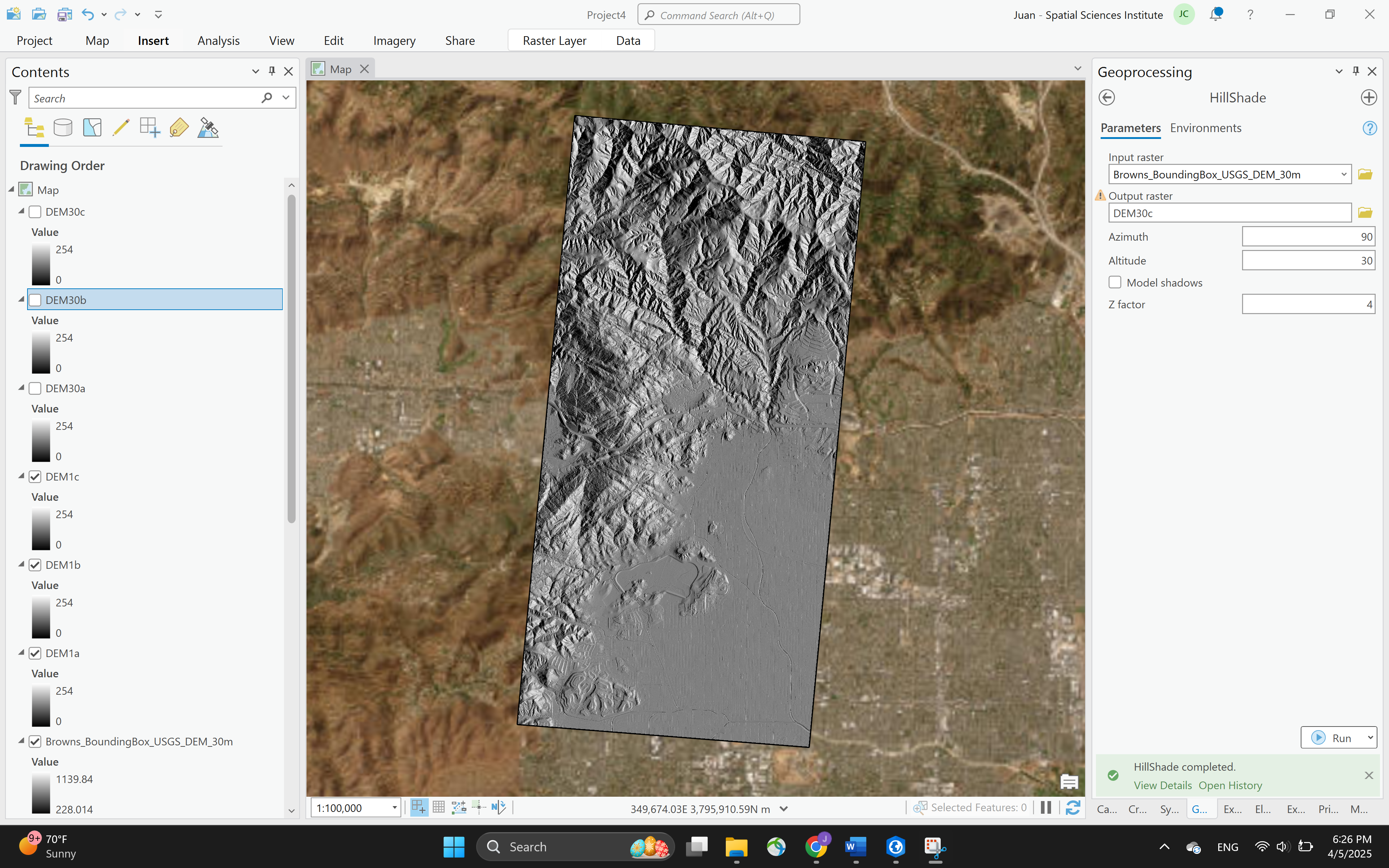
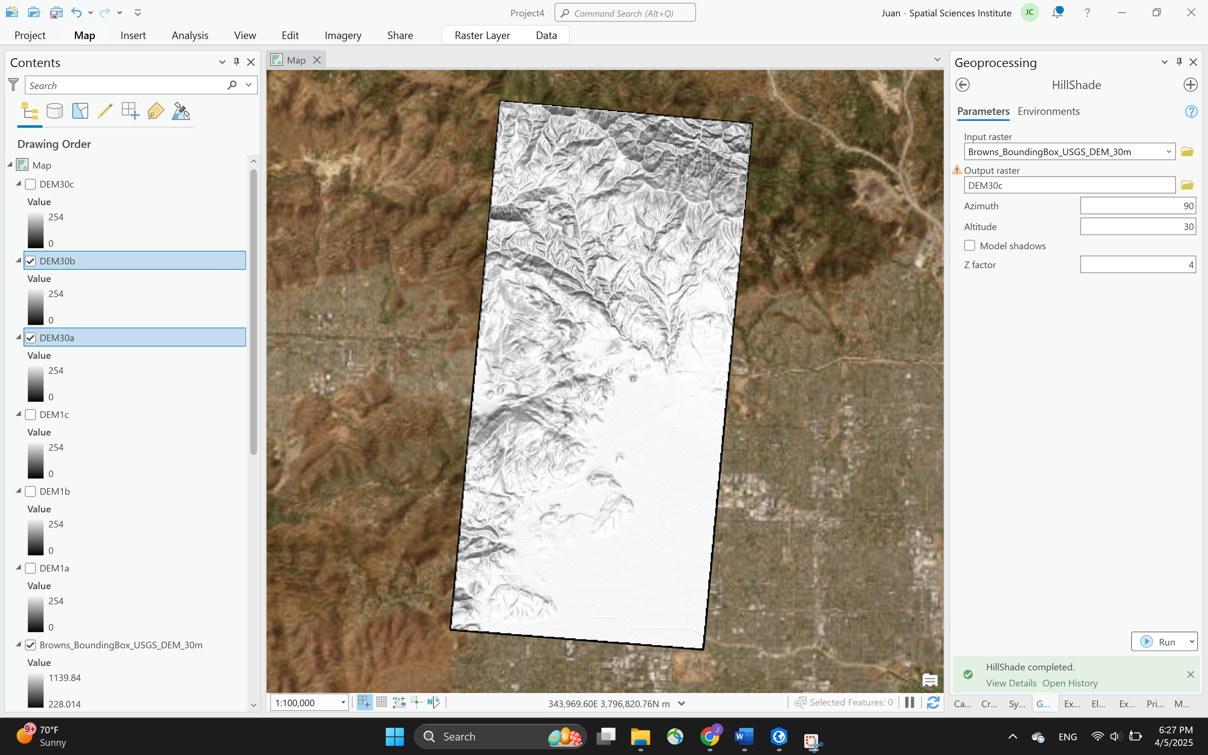
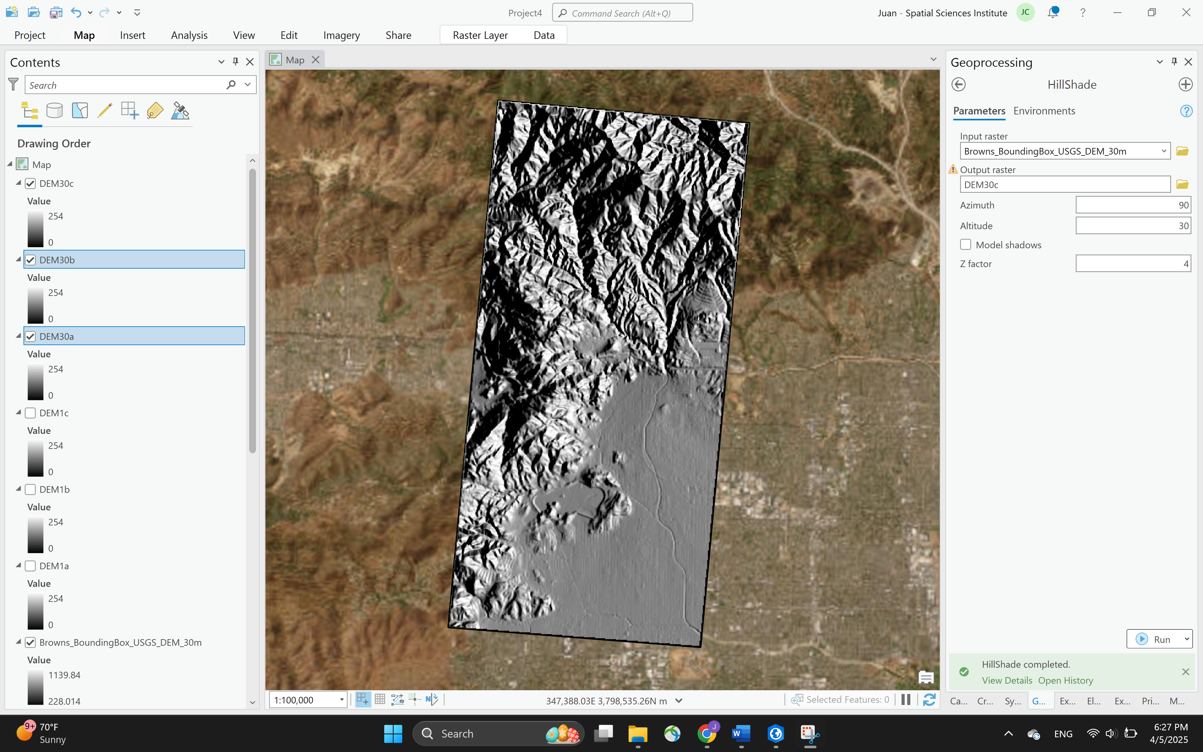
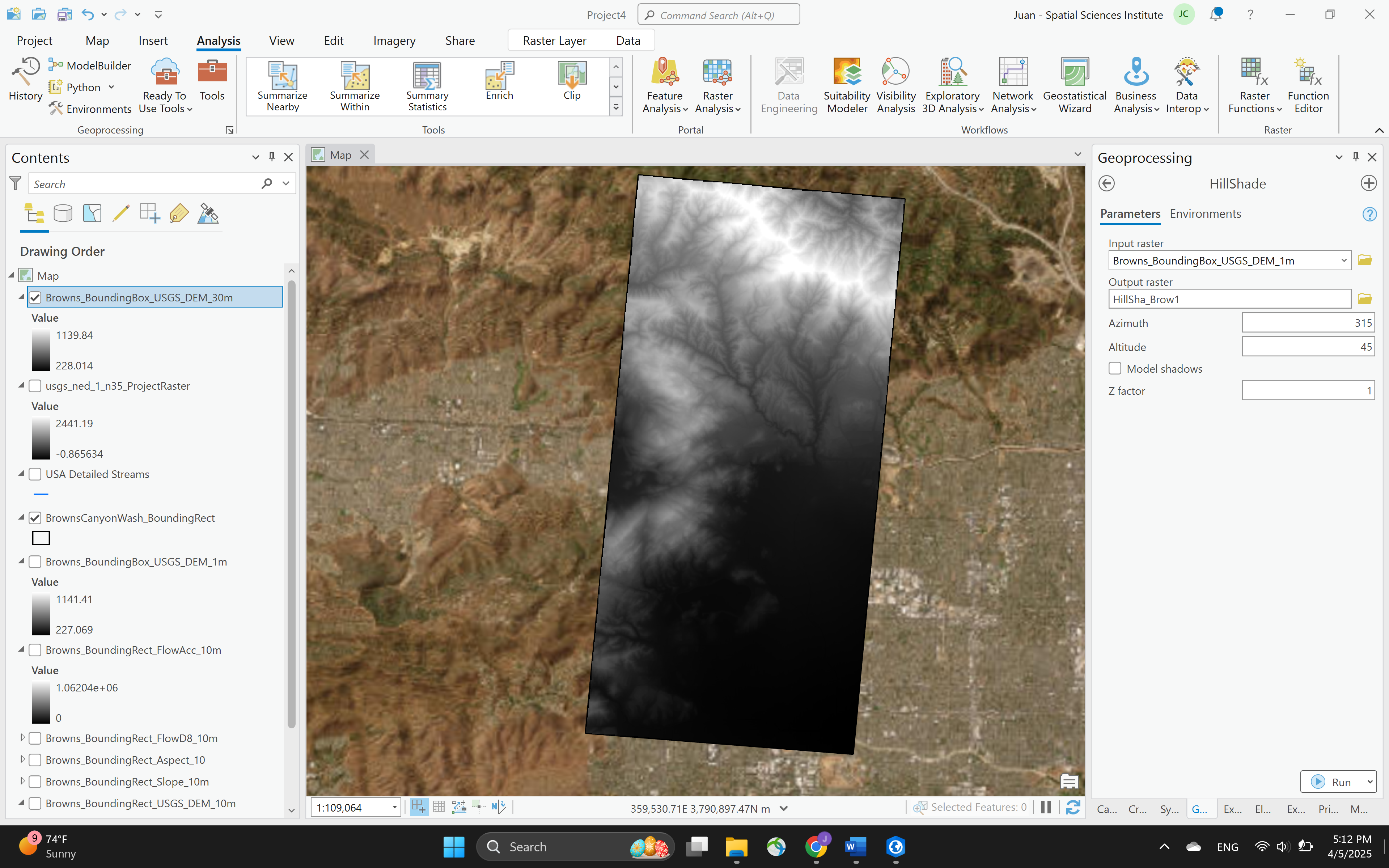
The Hillshade tool was applied to the 1m and 30m DEMs under six configurations simulating late afternoon, midday, and morning illumination. Azimuth, altitude, and Z-factor were adjusted to evaluate how different angles reveal or obscure terrain structure across Browns Canyon Wash.
| Setting | Late Afternoon (Default) | Midday Light | Morning Light | |||
|---|---|---|---|---|---|---|
| DEM 1m (a) | DEM 30m (a) | DEM 1m (b) | DEM 30m (b) | DEM 1m (c) | DEM 30m (c) | |
| Azimuth | 315° | 315° | 180° | 180° | 90° | 90° |
| Altitude | 45° | 45° | 75° | 75° | 30° | 30° |
| Z value | 1 | 1 | 1 | 2 | 1 | 4 |
DEM 1m (a) — Late Afternoon · Az 315° · Alt 45° · Z=1
DEM 30m (a) — Late Afternoon · Az 315° · Alt 45° · Z=1
DEM 1m (b) — Midday · Az 180° · Alt 75° · Z=1
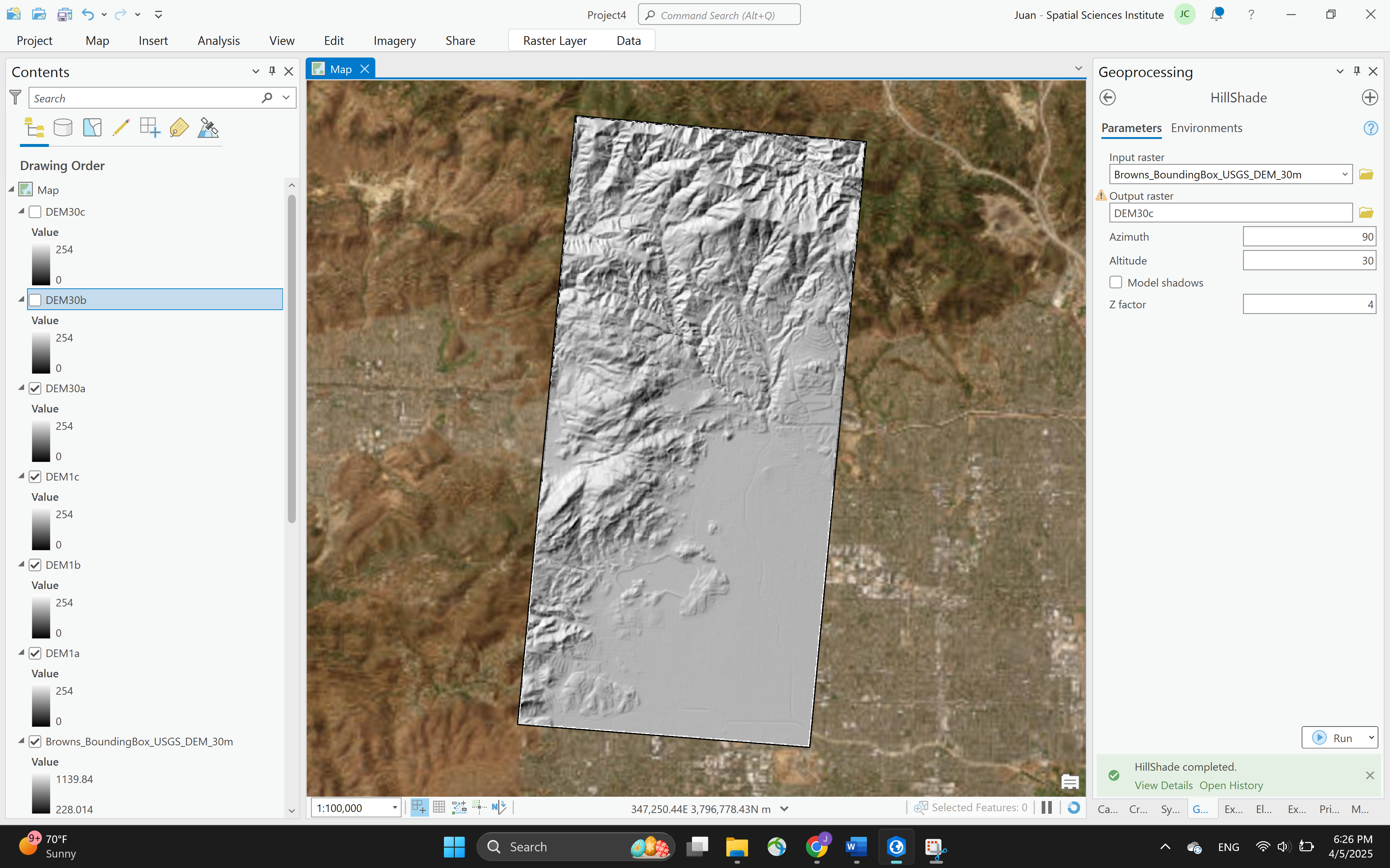
DEM 30m (b) — Midday · Az 180° · Alt 75° · Z=2
DEM 1m (c) — Morning · Az 90° · Alt 30° · Z=1
DEM 30m (c) — Morning · Az 90° · Alt 30° · Z=4
Increasing the Z value exaggerates elevation relief — most effective for the 30m DEM where generalization otherwise flattens subtle canyon structure. The morning light configuration (low altitude, eastward azimuth) produced the highest contrast on north-facing slopes, best revealing ridge-and-valley geometry across the Santa Susana Mountains.
Slope Analysis — Z-Factor Comparison
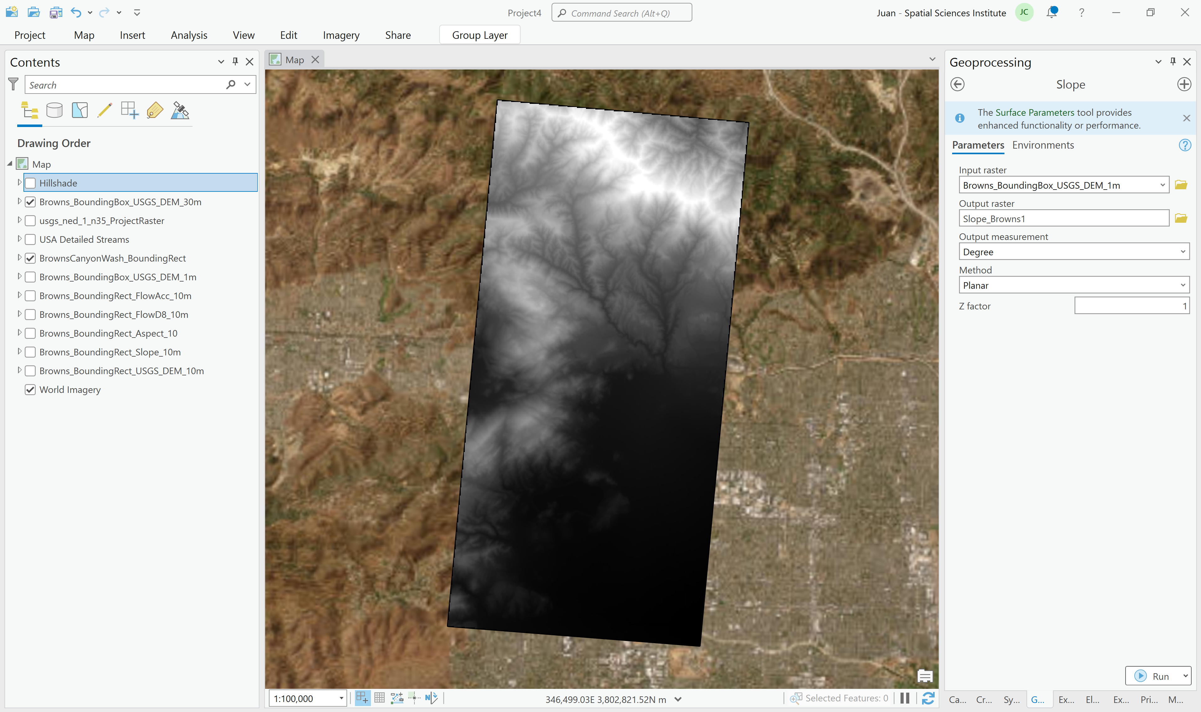
Slope was derived in degrees using the planar method. The Z factor was varied from 1 to 3 at both DEM scales to assess how vertical exaggeration affects gradient visualization across the canyon's steep terrain and flatter alluvial fan.
| Setting | DEM 1m | DEM 30m | DEM 1m (Z=3) | DEM 30m (Z=3) |
|---|---|---|---|---|
| Z factor | 1 | 1 | 3 | 3 |
DEM 1m slope — Z=1. Fine-grained micro-terrain detail captures narrow ridges and small-scale gradient changes.
DEM 1m slope — Z=3. Vertical exaggeration increases contrast on steeper slopes but amplifies visual complexity.
DEM 30m slope — Z=1. Dominant gradient zones are clearly legible without micro-terrain noise.
DEM 30m slope — Z=3. Exaggeration at coarser resolution sharpens the contrast between canyon walls and the flat valley floor without introducing noise.
Hydrologic Workflow & Troubleshooting
Each DEM was processed through a standard hydrologic modeling pipeline: Fill → Flow Direction → Flow Accumulation → Pour Point Placement → Watershed Delineation. Two significant technical challenges were encountered and resolved during this process.
-
01
Fill — Sink Removal
Applied to remove spurious sinks before flow direction modeling. On the 1m DEM, Fill initially returned NoData values across the raster — persisting through multiple reformatting attempts via the Copy Raster tool and NoData parameter adjustments. Fully resolved by updating ArcGIS Pro to the latest version.
-
02
Flow Direction & Flow Accumulation
Flow direction and accumulation rasters derived from filled DEMs. Symbology thresholds were iteratively adjusted to suppress straight-line artifacts from urban street grids — straightforward at 30m resolution but demanding constant zoom-level adjustment at 1m due to overwhelming pixel-level detail.
-
03
Pour Point Placement
Pour points placed at the highest-value cell in the Flow Accumulation raster — the outlet where Browns Canyon Creek joins the Los Angeles River. At 1m resolution, river channel alignment was noticeably offset from the 10m/30m outputs and the USGS reference shapefile, requiring visual approximation for accurate outlet cell identification.
-
04
Watershed Delineation
Initial single-point pour point attempts failed repeatedly — likely due to misalignment or snapping inaccuracies between the pour point layer and flow accumulation raster. Resolved by placing multiple points directly within the Watershed tool interface rather than from a separate point layer, ensuring each point corresponded to a verified high-flow cell.
ArcGIS Pro layer panel — all three DEM datasets loaded alongside flow direction, accumulation, and watershed outputs.
Flow accumulation raster — classification thresholds adjusted to isolate natural drainage paths from urban street-grid artifacts.
Watershed tool execution — multiple pour points placed on verified high-flow cells to bypass the initial delineation failure.
Pixel-to-area calculation — the highest-value flow accumulation pixel converted to watershed contributing area using (PV × 900) ÷ 1,000,000.
Watershed Area — Pixel Value Conversion
The highest-value cell in each Flow Accumulation raster marks the watershed outlet and was used to calculate approximate contributing area. The formula (pixel value × 900) ÷ 1,000,000 converts cell counts to km² for each resolution.
| DEM Resolution | Pixel Value | Area (km²) |
|---|---|---|
| DEM 1m | 40,071,388 | 40.07 km² |
| DEM 10m | 620,370 | 62.04 km² |
| DEM 30m | 69,697 | 62.73 km² |
The 1m DEM underestimates watershed area (~40 km²) compared to the 10m and 30m results (~62 km²), most likely due to river channel alignment offsets that shifted the pour point away from the true outlet. The 10m and 30m area estimates are highly consistent, reinforcing the 10m DEM as the most reliable reference for hydrologic computation at this scale.
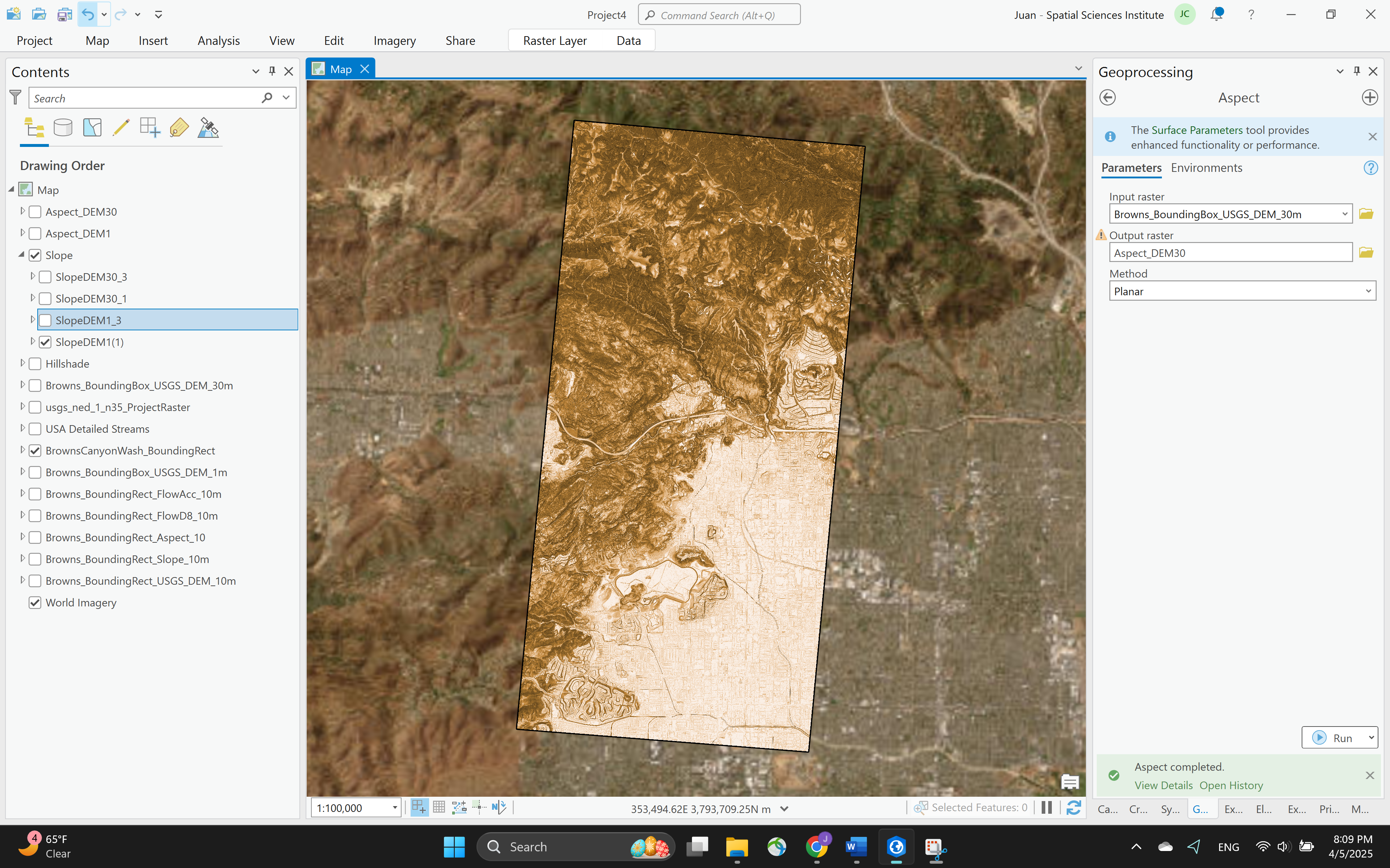
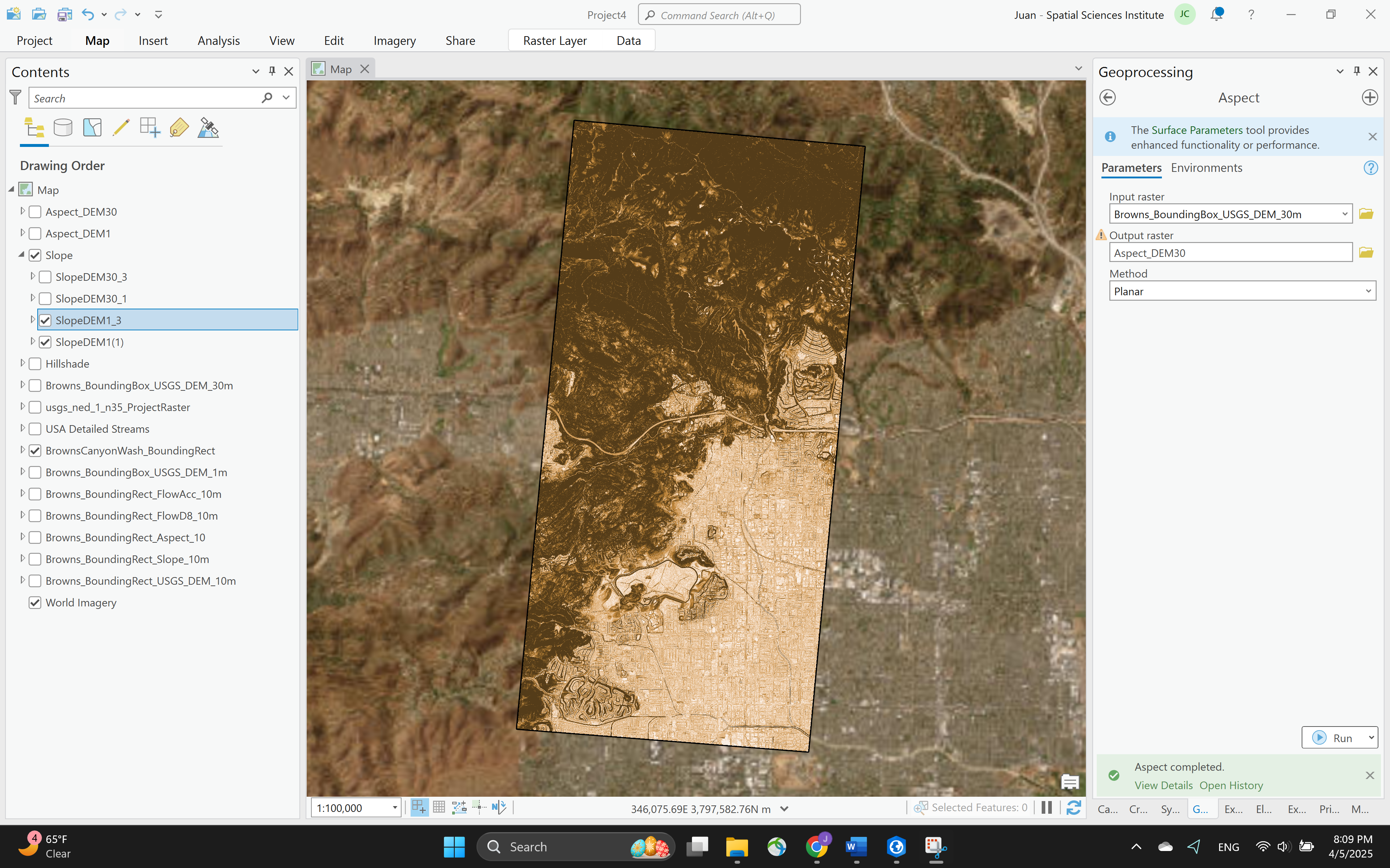
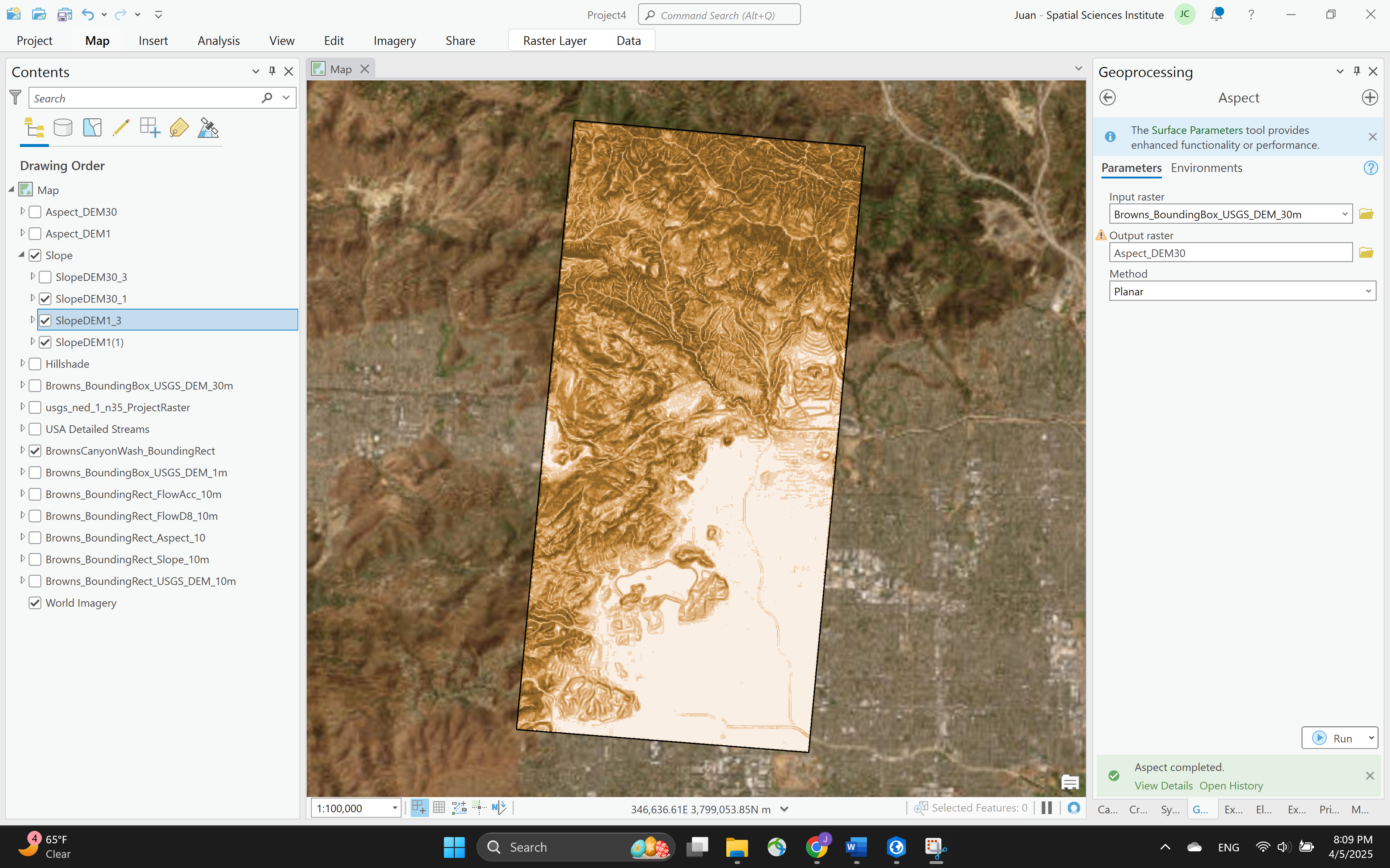
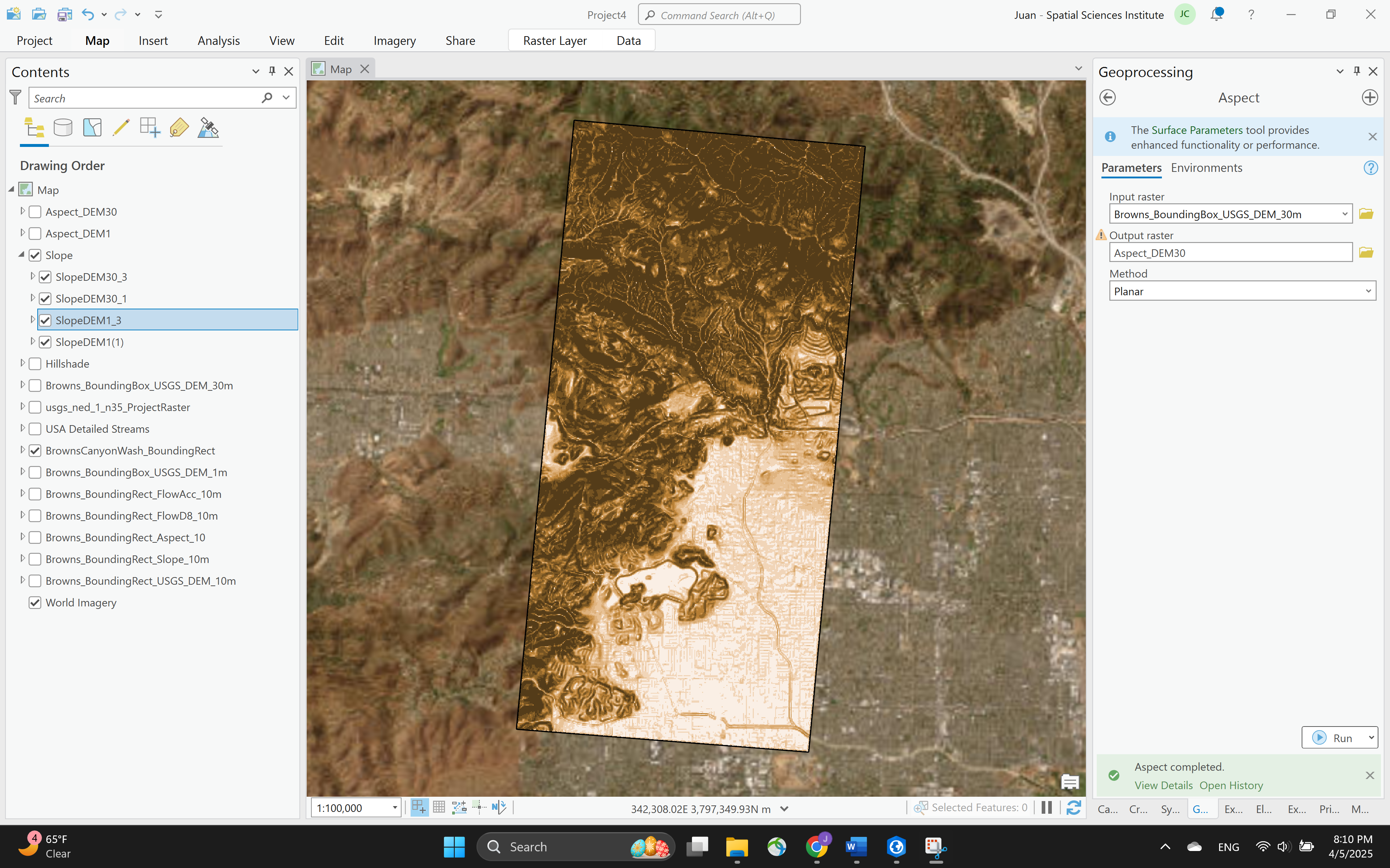
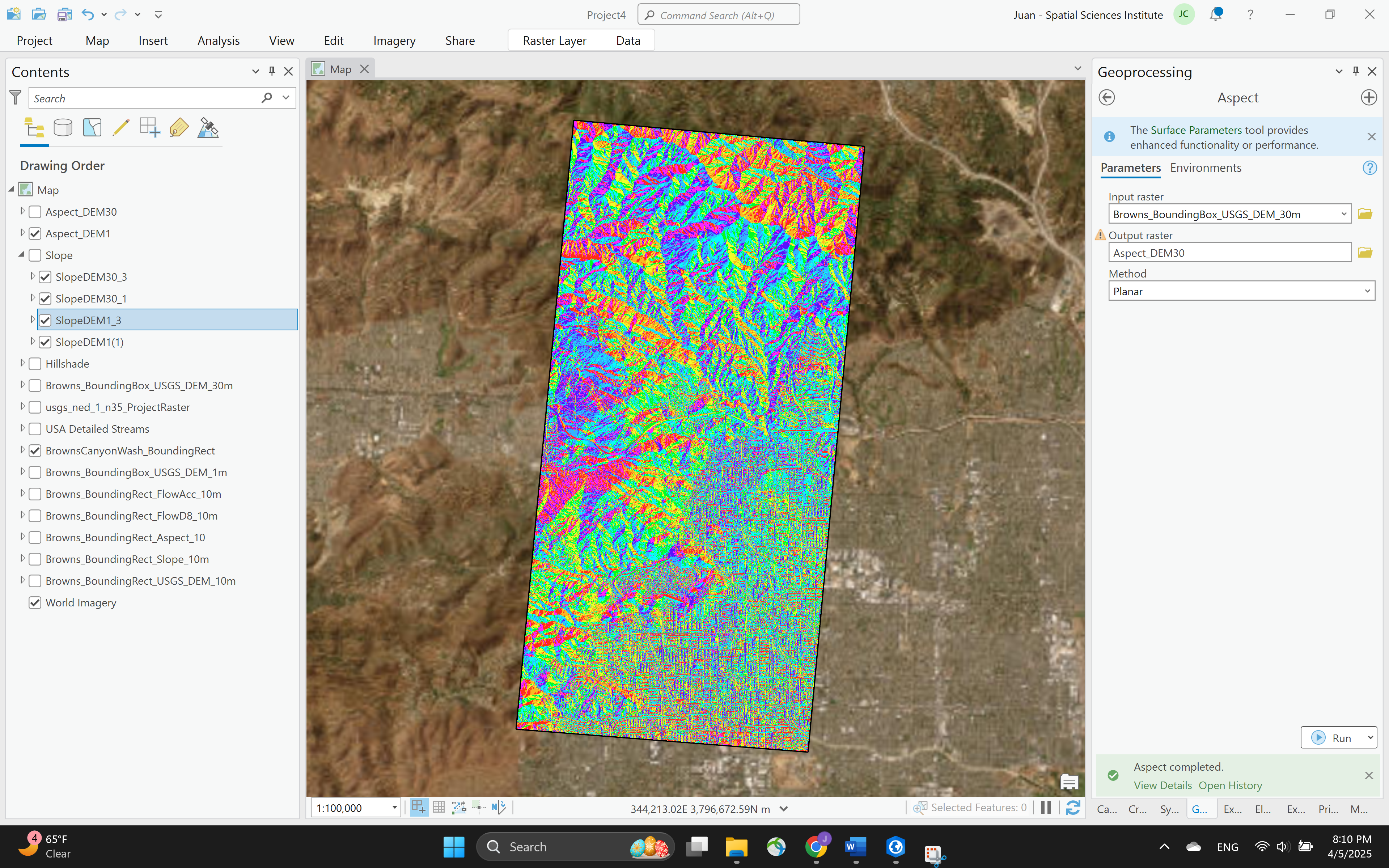
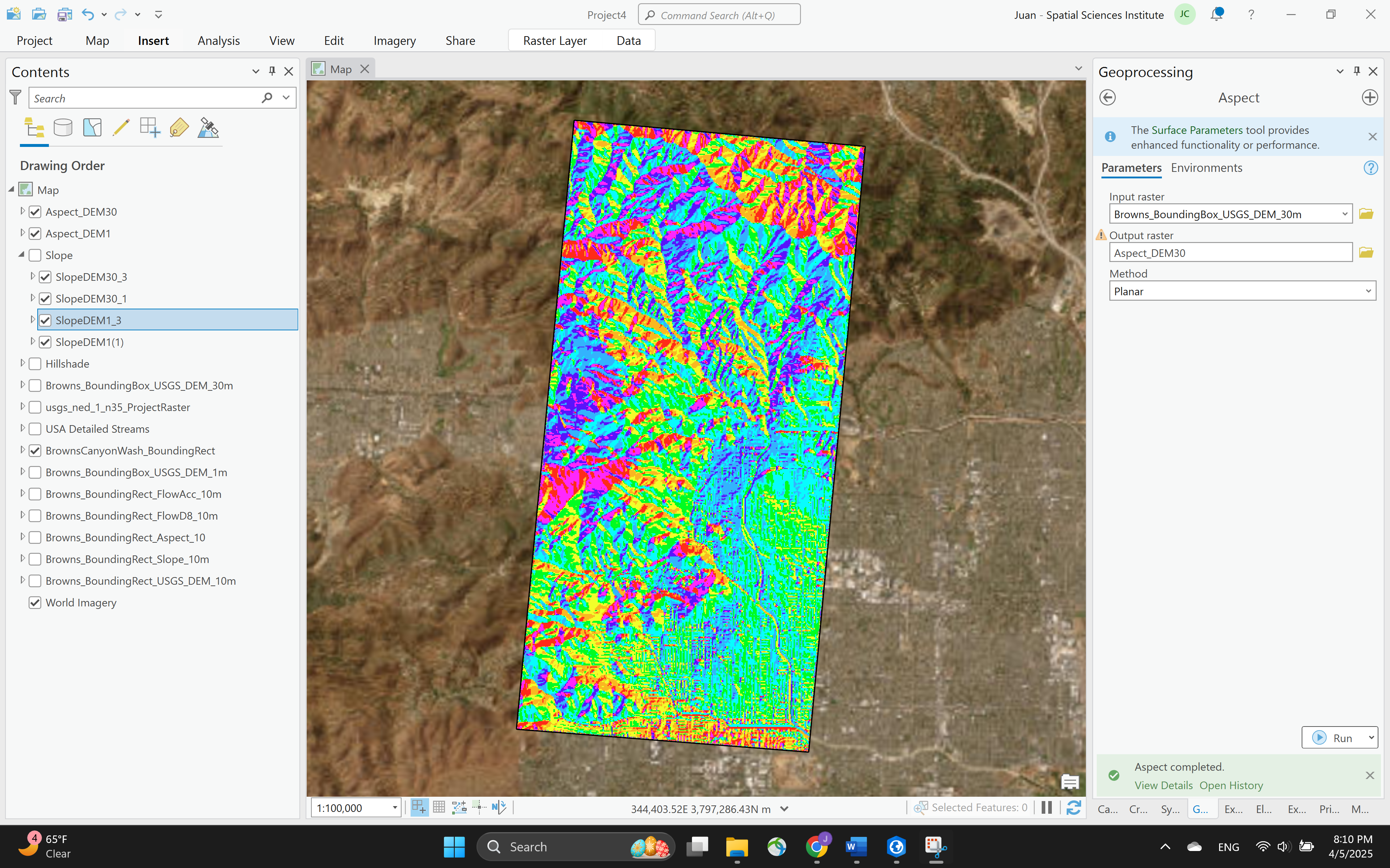
Results — Aspect Maps (1m · 10m · 30m)
Aspect maps illustrate slope orientation across Browns Canyon and reveal how resolution affects the clarity and fragmentation of directional terrain data. The 1m output captures highly fragmented slope orientations with micro-terrain precision, but at the cost of visual clarity. The 10m map strikes the most readable balance — clearly distinguishing ridge and valley slope directions without noise. The 30m map smooths orientations further, losing fine structure but enhancing interpretability at regional scale.
Aspect maps derived from the 30m, 10m, and 1m DEMs (top to bottom). The 10m output provides the clearest distinction between dominant ridge and valley slope orientations across the Santa Susana Mountains study area.
Results — Watershed Delineation (1m · 10m · 30m)
Watershed boundaries at three resolutions reveal how DEM scale directly affects hydrologic delineation quality. The 1m boundary is irregular and over-detailed, reflecting fine-resolution sensitivity to micro-terrain variations. The 10m watershed aligns closely with USGS reference data and provides the most consistent, reliable geometry. The 30m boundary effectively generalizes the drainage network extent, but produces a pixelated boundary appearance at standard map scales.
Watershed boundary comparisons at 30m, 10m, and 1m resolutions (top to bottom). Coarser DEMs show increased boundary smoothness and closer alignment with USGS reference shapefiles — finer resolution does not always yield better hydrologic interpretation.
The 10m DEM yielded the most consistent watershed geometry: clearer flow pathways with minimal breaks, reliable alignment with USGS reference data, and a clean, interpretable cartographic output. The 30m result captured the main drainage pattern but its pixelated boundary reduces its suitability for presentation-quality maps.
Discussion
Among the three DEMs, the 10m dataset proved the most balanced choice for both terrain and hydrologic analysis — minimizing noise while preserving relevant topographic detail, and aligning closely with established USGS reference workflows. The 1m DEM introduced significant preprocessing challenges and is better suited to high-precision work over smaller study extents. The 30m DEM, though computationally efficient, was too coarse for detailed terrain interpretation or presentation-quality output.
These results reflect the modifiable areal unit problem (MAUP): changes in raster resolution directly impacted watershed boundary interpretation, slope gradient clarity, and the reliability of pour point placement. Matching DEM scale to project scope and analysis objectives is essential — finer resolution amplifies detail but also error sensitivity, while coarser resolution trades precision for computational manageability. The 10m resolution successfully balanced these competing demands across all workflow components at the Browns Canyon Wash study area.
Limitations
- 1m DEM river alignment offset. At 1m resolution the flow accumulation channel was noticeably misaligned relative to the 10m/30m outputs and the USGS reference shapefile. Pour point placement at 1m relied on visual approximation, contributing to the lower watershed area estimate.
- Urban street grid artifacts. Flow accumulation rasters — especially at 1m — captured urban street grids as high-accumulation linear features. Iterative threshold adjustment suppressed most artifacts, but some straight-line features may persist in the final flow network.
- Fill tool NoData failure (1m DEM). The Fill tool initially produced NoData across the 1m raster. Though resolved by updating ArcGIS Pro, this underscores the importance of software currency when running computationally intensive tools on high-resolution inputs.
- 30m pixelation. The 30m watershed boundary has a coarse, pixelated appearance at map scale, limiting its utility for high-quality cartographic output — despite adequately representing the overall drainage network extent.